SEO data analysis
This blog post is published first on 2018-10-18 and updated on 2019-08-20.
This blog post and the jupyter notebook aim to answer the following questions:
1) Decide whether diffferent collected SEO data are correlated.
2) How many days of web server logs are needed to calculate certain SEO metrics.
3) Identify the trend, seasonality in each collected SEO data.
Jupyter notebook is available at SEO Data Analysis Notebook
Collected SEO data
crawl.csv : Crawled pages data(crawled by googlebot) collected between 2016 and 2019.
'crawl unique' : For a specific page on a day, this column value is equal to 1, if this page is crawled at least once by googlebot on that day.
active.csv: Active pages data(google search engine) between 2016 and 2019
'active unique' : For a specific page on a day, this column value is equal to 1, if this page receives at least one visit from google on that day.
SEO data analysis
First import the necessary python libraries
import pandas as pd
from sklearn.preprocessing import MinMaxScaler
import matplotlib.pyplot as plt
%matplotlib inline
from statsmodels.tsa.seasonal import seasonal_decompose
Read the SEO data in files into pandas dataframes
df_crawl = pd.read_csv('crawl.csv',parse_dates=['date'], index_col='date')
df_active = pd.read_csv('active.csv',parse_dates=['date'], index_col='date')
Resample, scale, plot daily SEO data
df_sum_crawl = df_crawl.resample('D').sum()
df_sum_active = df_active.resample('D').sum()
df_sum = pd.concat([df_sum_crawl['crawl unique'],df_sum_active['active unique']],axis=1)
scaler = MinMaxScaler()
df_sum[['crawl unique', 'active unique']] = scaler.fit_transform(df_sum[['crawl unique', 'active unique']])
df_sum[['crawl unique','active unique']].plot(figsize=(15,8));
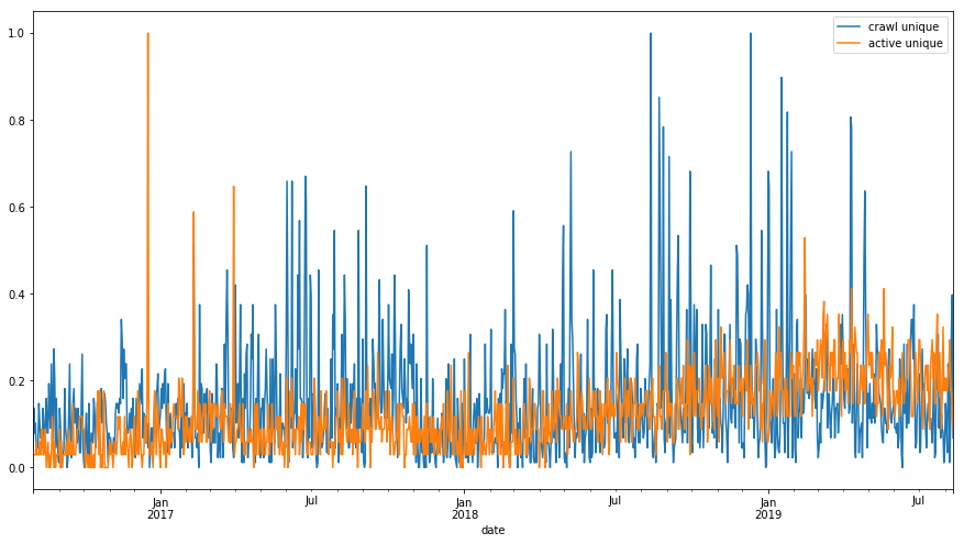
Check the correlations of resampled daily SEO data
df_sum.corr()
crawl unique active unique
crawl unique 1.00000 0.143273
active unique 0.143273 1.00000
Resample, scale, plot weekly SEO data
df_sum_crawl = df_crawl.resample('W').sum()
df_sum_active = df_active.resample('W').sum()
df_sum = pd.concat([df_sum_crawl['crawl unique'],df_sum_active['active unique']],axis=1)
scaler = MinMaxScaler()
df_sum[['crawl unique', 'active unique']] = scaler.fit_transform(df_sum[['crawl unique', 'active unique']])
df_sum[['crawl unique','active unique']].plot(figsize=(15,8));
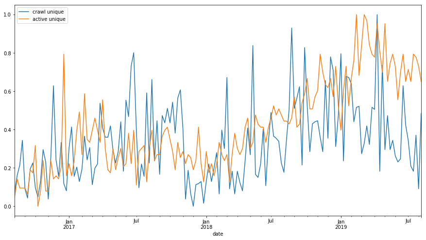
Check the correlations of resampled weekly SEO data
df_sum.corr()
crawl unique active unique
crawl unique 1.000000 0.34085
active unique 0.34085 1.000000
Resample, scale, plot biweekly SEO data
df_sum_crawl = df_crawl.resample('SMS').sum()
df_sum_active = df_active.resample('SMS').sum()
df_sum = pd.concat([df_sum_crawl['crawl unique'],df_sum_active['active unique']],axis=1)
scaler = MinMaxScaler()
df_sum[['crawl unique', 'active unique']] = scaler.fit_transform(df_sum[['crawl unique', 'active unique']])
df_sum[['crawl unique','active unique']].plot(figsize=(15,8));
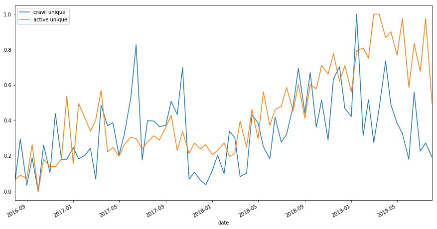
Check the correlations of resampled biweekly SEO data
df_sum.corr()
crawl unique active unique
crawl unique 1.000000 0.463403
active unique 0.463403 1.000000
Resample, scale, plot monthly SEO data
df_sum_crawl = df_crawl.resample('M').sum()
df_sum_active = df_active.resample('M').sum()
df_sum = pd.concat([df_sum_crawl['crawl unique'],df_sum_active['active unique']],axis=1)
scaler = MinMaxScaler()
df_sum[['crawl unique', 'active unique']] = scaler.fit_transform(df_sum[['crawl unique', 'active unique']])
df_sum[['crawl unique','active unique']].plot(figsize=(15,8));
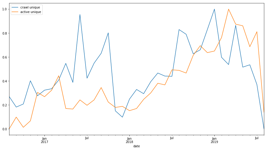
Check the correlations of resampled monthly SEO data
df_sum.corr()
crawl unique active unique
crawl unique 1.000000 0.525298
active unique 0.525298 1.000000
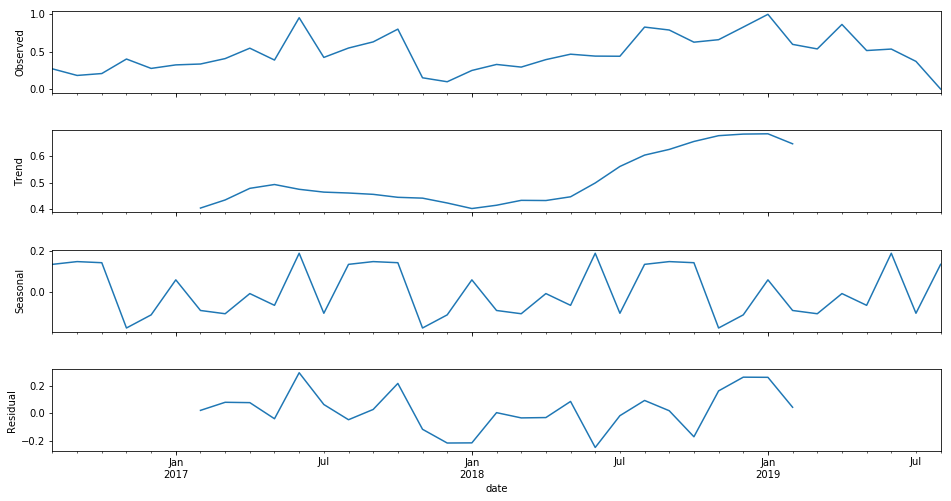
Observed, trend, seasonal, residual data analysis of monthly crawled pages SEO data
decomposition = seasonal_decompose(df_sum['crawl unique'], freq = 12) fig = plt.figure() fig = decomposition.plot() fig.set_size_inches(15, 8);
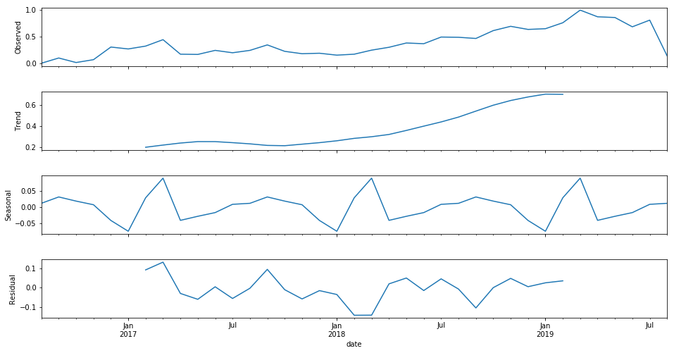
Observed, trend, seasonal, residual data analysis of monthly active pages SEO data
decomposition = seasonal_decompose(df_sum['active unique'], freq = 12) fig = plt.figure() fig = decomposition.plot() fig.set_size_inches(15, 8)

SEO data analysis results
Concerning collected SEO data of this website:
1) There are correlations between the number of unique crawled pages by googlebot, unique active pages receiving organic traffic from google. All SEO data sources collected as datetime data later resampled to daily, weekly, biweekly and monthly data.
2) By looking at the correlation results, we can assume that If we would like to calculate some SEO metrics, we need at least one week of crawled and active pages data. However to have more accurate and actual results, it is better to perform correlation analysis in recent years or months and with unique crawled pages in 200 HTTP status code rather than on all unique crawled pages. Here, the estimated time frame as a week is a very rough estimate. Also this is an estimation for the site globally. Different categories on the site may require different days of logs in order to calculate their SEO metrics effectively.
3) As a trend we see an increase on both number of unique crawled pages and unique active pages.
4) There is seasonality on both crawled and active pages.
Next blog post following to this one is about forecasting SEO data which is available at URL SEO Data Forecasting
Thanks for taking time to read this post. I offer consulting, architecture and hands-on development services in web/digital to clients in Europe & North America. If you'd like to discuss how my offerings can help your business please contact me via LinkedIn
Have comments, questions or feedback about this article? Please do share them with us here.
If you like this article


Comments