SEO Forecasting

This blog post is published first on 2018-10-22  and updated on 2023-03-07.

With supervised machine learning, it is possible to solve mainly two types of problems which are prediction and classification.

In this blog post, using a time-series machine learning model, pmdarima's auto-arima, over three years of collected SEO data, I will predict a site's monthly active pages.

This blog post and jupyter notebook aims to answer the following questions:

1) Can we predict SEO data with other related SEO data that we know is correlated?

2) How to evaluate predicted SEO results?

3) How can we use this model and the predicted SEO results?

Jupyter Notebook is available at SEO forecasting notebook

Collected SEO data

crawl.csv :  Crawled pages data(crawled by googlebot) collected  between 2016 and 2019. 

'crawl unique'  : For a specific page on a day,  this column value is equal to 1, if this page is crawled at least once by googlebot on that day. 

active.csv: Active pages data(google search engine) between 2016 and 2019

'active unique' : For a specific page on a day, this column value is equal to 1, if this page receives at least one visit from google on that day.

SEO data analysis

This part is treated in the previous blog post  SEO data analysis

SEO forecasting: Forecasting monthly crawled pages

First import the necessary python libraries

import pandas as pd
import numpy as np
import matplotlib.pyplot as plt
import pmdarima as pm
%matplotlib inline
from sklearn.preprocessing import MinMaxScaler

Read the SEO data in files into  pandas dataframe

scaler = MinMaxScaler()
df_crawl = pd.read_csv("crawl.csv",parse_dates=['date'], index_col='date')
df_active = pd.read_csv('active.csv',parse_dates=['date'], index_col='date')
df_sum_crawl = df_crawl['2016-08-01':'2019-07-31'].resample('M').sum()
df_sum_active = df_active['2016-08-01':'2019-07-31'].resample('M').sum()
data = pd.concat([df_sum_crawl['crawl unique'],df_sum_active['active unique']],axis=1)
data[['crawl unique', 'active unique']] = scaler.fit_transform(data[['crawl unique', 'active unique']])

Split the SEO data to train and test SEO data sets. Our target SEO variable is active pages, our exogenous SEO variable is the crawled pages. Seasonal set to True, stepwise=True in modeling. 

# #############################################################################
# Load the data and split it into separate pieces

train, test = data[:29], data[29:]

# Fit a simple auto_arima model
forecast_active_pages = pm.auto_arima(y=train['active unique'], exogenous=train["crawl unique"].values.reshape(-1, 1), trace=1,
seasonal=True,
error_action='ignore', # don't want to know if an order does not work
suppress_warnings=True, # don't want convergence warnings
stepwise=True)

print(forecast_active_pages.summary())

Fit ARIMA: order=(2, 1, 2) seasonal_order=(0, 0, 0, 1); AIC=-54.692, BIC=-45.366, Fit time=0.384 seconds
Fit ARIMA: order=(0, 1, 0) seasonal_order=(0, 0, 0, 1); AIC=-45.793, BIC=-41.797, Fit time=0.073 seconds
Fit ARIMA: order=(1, 1, 0) seasonal_order=(0, 0, 0, 1); AIC=-44.850, BIC=-39.521, Fit time=0.057 seconds
Fit ARIMA: order=(0, 1, 1) seasonal_order=(0, 0, 0, 1); AIC=-45.530, BIC=-40.202, Fit time=0.093 seconds
Fit ARIMA: order=(1, 1, 2) seasonal_order=(0, 0, 0, 1); AIC=-47.668, BIC=-39.674, Fit time=0.294 seconds
Fit ARIMA: order=(3, 1, 2) seasonal_order=(0, 0, 0, 1); AIC=-50.596, BIC=-39.939, Fit time=0.396 seconds
Fit ARIMA: order=(2, 1, 1) seasonal_order=(0, 0, 0, 1); AIC=-52.664, BIC=-44.671, Fit time=0.354 seconds
Fit ARIMA: order=(2, 1, 3) seasonal_order=(0, 0, 0, 1); AIC=-57.754, BIC=-47.096, Fit time=0.414 seconds
Fit ARIMA: order=(3, 1, 4) seasonal_order=(0, 0, 0, 1); AIC=-54.710, BIC=-41.388, Fit time=0.532 seconds
Fit ARIMA: order=(1, 1, 3) seasonal_order=(0, 0, 0, 1); AIC=-47.499, BIC=-38.174, Fit time=0.406 seconds
Fit ARIMA: order=(3, 1, 3) seasonal_order=(0, 0, 0, 1); AIC=-56.027, BIC=-44.038, Fit time=0.448 seconds
Fit ARIMA: order=(2, 1, 4) seasonal_order=(0, 0, 0, 1); AIC=-55.863, BIC=-43.873, Fit time=0.561 seconds
Total fit time: 4.029 seconds
 Statespace Model Results 
==============================================================================
Dep. Variable: y No. Observations: 29
Model: SARIMAX(2, 1, 3) Log Likelihood 36.877
Date: Sun, 01 Sep 2019 AIC -57.754
Time: 14:12:35 BIC -47.096
Sample: 0 HQIC -54.496
 - 29 
Covariance Type: opg 
==============================================================================
 coef std err z P>|z| [0.025 0.975]
------------------------------------------------------------------------------
intercept 0.0673 0.054 1.243 0.214 -0.039 0.173
x1 -0.0737 0.040 -1.824 0.068 -0.153 0.005
ar.L1 -0.7561 0.148 -5.111 0.000 -1.046 -0.466
ar.L2 -0.8696 0.161 -5.391 0.000 -1.186 -0.553
ma.L1 0.9385 0.346 2.716 0.007 0.261 1.616
ma.L2 1.0481 0.413 2.539 0.011 0.239 1.857
ma.L3 0.6983 0.537 1.300 0.194 -0.355 1.751
sigma2 0.0036 0.002 2.002 0.045 7.6e-05 0.007
===================================================================================
Ljung-Box (Q): nan Jarque-Bera (JB): 2.70
Prob(Q): nan Prob(JB): 0.26
Heteroskedasticity (H): 0.44 Skew: -0.57
Prob(H) (two-sided): 0.24 Kurtosis: 4.00
===================================================================================

# #############################################################################
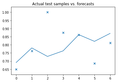
# Plot actual test vs. forecasts:
x = np.arange(test['active unique'].shape[0])
plt.scatter(x, test['active unique'], marker='x')
plt.plot(x, forecast_active_pages.predict(exogenous=test['crawl unique'].values.reshape(-1, 1),n_periods=test.shape[0]))
plt.title('Actual test samples vs. forecasts')
plt.show();

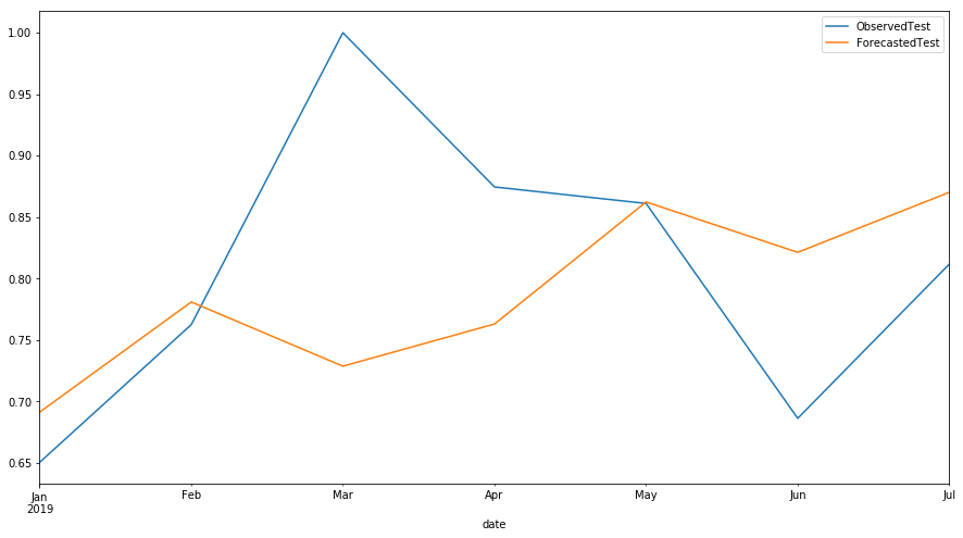
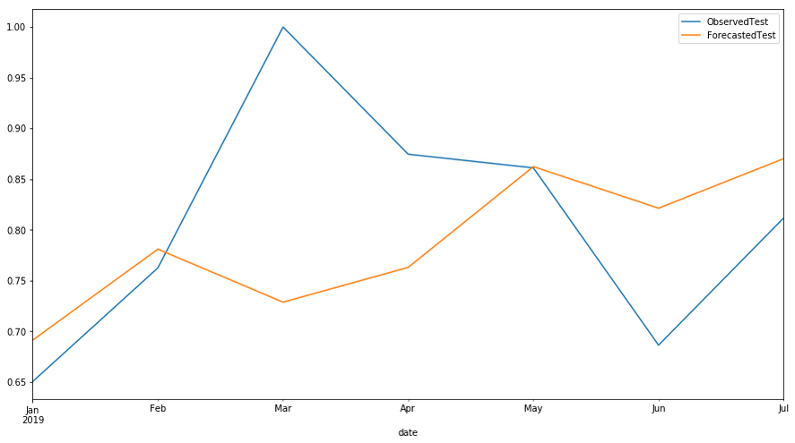
Forecast SEO data in our case, volume of monthly resampled daily active pages in 2019 and plot observed vs forecasted data 

predicts = pd.DataFrame(forecast_active_pages.predict(exogenous=test['crawl unique'].values.reshape(-1, 1),n_periods=test.shape[0]), index = test.index)
pd.concat([test['active unique'],predicts],axis=1).plot(figsize=(15,8))
L=plt.legend()
L.get_texts()[0].set_text('ObservedTest')
L.get_texts()[1].set_text('ForecastedTest')

SEO Forecasting results

Regarding the prediction of this website's SEO data:

1) In the previous blog post on SEO data analysis, it was found that there are correlations between the number of unique pages crawled by googlebot and the unique active pages receiving organic traffic from google. All SEO data sources collected as datetime data later resampled to monthly data.

2) In the previous blog post on SEO data analysis, seasonality is detected on crawl and active data. Therefore, in the model, seasonal is set to True.

3) The model created above is not optimized so the predictions are not accurate. In order to optimize the model, we have several options e.g. we can recreate the model with unique crawled pages in HTTP status code 200. The model can also be optimized by hyperparameter tuning.

4) More exogenous SEO variables can be added to the model if found to be correlated with the target variable, such as marketing spend, google trending data of keywords important to the website, average website ranking on google for these important keywords etc

5) The model can be used to evaluate our SEO work. If, for example, the predicted number of active pages and the error measure of the number of active pages observed give very different results from previous ones where there is no SEO work, it can be assumed that there is had a hidden variable, most likely an "SEO job"

6) As we forecast the number of monthly unique active pages, the number of monthly unique crawled pages on a site can also be forecast. This can help us identify anomalies in the number of crawled pages; decrease or increase over time and whether they are expected or unexpected behaviors.

Thanks for taking time to read this post. I offer consulting, architecture and hands-on development services in web/digital to clients in Europe & North America. If you'd like to discuss how my offerings can help your business please contact me via LinkedIn

Have comments, questions or feedback about this article? Please do share them with us here.

If you like this article

Follow Me on Twitter

Follow Searchdatalogy on Twitter